From this post onwards, we will be covering advanced algorithms in javascript. We are going to learn about dynamic programming. The definition of this algorithm is a little abstract, and the best way to understand it, is to see it in action. My goal is to make this a great resource for learning how to implement dynamic programming problems in javascript. To understand this algorithm we must first try to understand what optimization problems are. Why? Let’s start off with dynamic programming, which is a way of solving optimization problems by breaking them into smaller subproblems. From the definition above (Wikipedia link), we see that an optimization problem is the problem of finding the best solution, from all feasible solutions. Generally, there are quite a few ways for going about finding best solutions to these problems. One common way might be through enumeration, where you find all possible solutions, and pick one – the most optimal. For example, if I asked for the number of ways to climb 3 steps (staircase), you might have to go through an enumeration process to give me that answer. Another way of solving optimization problems might be to find a feasible solution that minimizes (or maximizes) the problem. Think about a problem where we want to maximize the area of a field (for e.g finding the largest possible rectangular area you can enclose), given that we can only use a 1000 ft of fencing material. Or perhaps find the max money you have made from buying and selling a stock given a number of days. There are optimization problems where we need to answer a yes or no for a given problem (for e.g. can you get 5 dollars from X amount of dimes and Y amount quarters). Optimization problems allow you explore all possible solutions by breaking problems into small sub-problems and then you build up solutions to bigger sub-problems. All we are doing is making a set of choices so we can arrive at an optimal solution.

Dynamic programming is sometimes considered the reverse of recursion. We have seen recursion already in previous posts. Instead of starting from the top and breaking the problem down into smaller sub-problems, this time we start from the bottom and we solve those small problems first and combine them to solve a larger problem. As a matter of fact, you can rewrite many recursive solutions using dynamic programming (you will be seeing a lot of examples of these here). Why? As elegant as recursive solutions are, they can be quite taxing depending on the programming language you are implementing it in. Some languages don’t have good support for recursion. Don’t forget that the time complexity for a recursive function is exponential (log 2^n), which is not good. You can drastically reduce this to a complexity of log(N)! by using dynamic programming. This approach builds up a table (array-based) and store results of subproblems it encounters, and these results are accessible during program execution. It’s very cool! However dynamic programming can be tricky to implement. And one needs to practice extensively to get used to this type of approach to solving problems. I definitely cant say I am a master yet. The most important thing to remember is that we want to solve subproblems first and build up to solve bigger problems. We will see how its done when we start solving well known dynamic programming problems. Let’s get started!

Content List:

1. Fibonacci Numbers
2. Factorial
3. Climbing Stairs
4. Cutting Rods
5. House Robber
6. Buy/Sell Stock to Maximize Profit
7. Maximum Length Chain of Pairs
8. 0 – 1 Knapsack Problem
9. Longest Common Subsequence
10. Longest Common Substring
11. Maximum Sum Contiguous Subarray Problem

These are the problems we are going to be solving in this post. If you are new to dynamic programming I would suggest you started from #1 to the end. However, if you have some experience with this topic then feel free to jump to any question if that is what you are interested in.

Fibonacci Numbers

We all studied this in high school or college mathematics. They are a sequence of numbers generated by adding the previous two numbers in the sequence together.

0, 1, 1, 2, 3, 5, 8, 13, 21, 34, 55, 89, 144, …

Now that we know how these numbers are generated, let’s write a function that generates them. There are a few ways to do this. The first and intuitive way is using the iterative approach. Another approach is to use recursion, which is more advanced (and not intuitive – though elegant). I mentioned previously that you could implement most recursive functions using dynamic programming to get better performance results. This is the third way. We will also look at a special fourth way called memoization. While this method is similar to dynamic programming; it gives us a way to efficiently store already computed results so we don’t compute it again (the reason why recursion is not so efficient), it is different from dynamic programming. We will see why later. In computing, memoization is an optimization technique used primarily to speed up computer programs by storing the results of expensive function calls and returning the cached result when the same inputs occur again. When should you use it? When you are running expensive tasks in your program that you know can be cached for later retrieval. Let’s move on.

So why is recursion inefficient in some programming languages. Let’s see what happens when you call a function recursively.

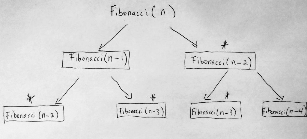
When we make recursive function calls, the problem is that we keep calling functions that have already run (they are not cached and thus have to be recalculated). Looking at the diagram, if we called the Fibonacci function for say N, we notice that during execution, the program splits up into different paths (this is also the top-down approach). Notice for example Fibonacci(n – 2) and Fibonacci(n – 3) is called more than once. For larger N values, can you imagine how big the function call stack will be? Functions that have already executed will be run again. So languages that are not built to handle such processes cannot efficiently run recursive programs. Javascript used to be one of those languages, HOWEVER as of ECMAScript 6, thanks to something called tail call optimization, recursion is not slower as compared to other programming languages that can’t handle recursion well. However, it is still a slow algorithm and runs at an exponential time complexity log(2^n). Let’s take a look at some code. We are going to write some Fibonacci functions that display the first N numbers in the sequence (or even calculate the sum total of the numbers). We will see which methods run the fastest.

See the Pen Fibonacci – Various solutions by kofi (@scriptonian) on CodePen.

We start off by solving the Fibonacci problem in an iterative approach. There are no tricks here. We gather all the ideas we know about the sequence. The declared variables represent the first 3 sequences. If we know 2 numbers we can find the third. We store the first two in an array and then we use the formula to generate the next number and the one after that in an iterative approach, pushing the result into an array. When all is said and done we return the array (which holds the number sequence to display). The second method recursiveFibonacci finds the number sequence using recursion. It is important to note that when n is 1 or 2, that value gets returned. This is the base case we always define when solving problems with recursion. Fibonacci of n = 1 is 1, and n = 2 is 2 (n is sequence number total). Notice how the base case is defined in the function. We will come back to this in a few. We repeatedly call the function N times, which slowly breaks up the problem into smaller and smaller parts on each call. When it cannot be broken any further we put it back together and return the final result. While this is the sum total, I have written code that returns the sequence as well. You can go ahead and run this to see the results. If you need code commenting, please check out the github repo for that. Next, we will take a look at the Dynamic Programming approach. Notice something different here? We stored our base cases in an array. Then we use a for-loop to calculate the next sequence. Now in order to get the next number (which we get by adding the previous two numbers), we don’t have to do that calculation at all (because we already stored it in the array – we simply retrieve it). What’s the runtime complexity of getting a number stored in an array index? Its O(1), which is very fast (constant time). When we run sequence[i] = sequence[i – 1] + sequence[i – 2], for i = 2, we get sequence[2] = sequence[1] + sequence[0]. We already know what sequence[1] and sequence[0] are. So we quickly retrieve them to get sequence[2] which is also stored in the 2nd index of the array. When we get to s[3], we already have s[2] and s[1]. We have used this approach to build an array which includes the solutions to our subproblems. When we are done we return the array to the caller. This solution runs at linear time O(N) because we run one loop from index of 3 to N. Notice this is way better than the recursive and iterative approach. The recursive approach also does other things like variable swapping. Finally, let us talk about the memoize function. Our memoize Fibonacci function returns a function that is the Fibonacci function we eventually call (closure). The function has access to a cache object. When Fibonacci is called we do pretty much the same thing that we did in the recursive solution with a little twist. Instead of repeatedly calling the function for every number, we check to see if that number/input has already been calculated(in cache). So for e.g, if we have Fibonacci for n = 10, why run it again? Instead, pull the result from the cache. This makes our function run much faster. Try running the code. You will notice that the dynamic approach runs the fastest, followed by the iterative approach, then the memoized approach and then the recursive solution is slowest (the others are about 6 times faster!). It may seem like memoization and dynamic programming are the same. But I can assure you they are different. The main difference being that memoization takes a top-down computation approach (similar to recursion) whereas dynamic programming takes a bottom-down. Again, note that the top-down approach is just the diagram I showed above for recursion, however, this is a more optimized approach where we cache results that are already computed. Between the two approaches, I would choose dynamic programming as its a bit faster. If you want to find out more, read this article.

What is the take away here? When solving problems using the dynamic programming approach we first start off by defining our base cases. We also define an array to store values in. Then instead of calling the function recursively, we run a loop to find out what the next case results in (based on previous base case values in an array).

Factorial

Here is another thing we studied in high school or college. A factorial is the product of a series of factors in an arithmetic progression. The formula is:

n! = n * (n – 1 ) * (n – 2) * (n – 3) * … * 2 * 1

Do you remember? You may have already seen the recursive solution to this problem. However, how can we use dynamic programming to our benefit? No need for a lot of theory on this one, lets just jump straight into code.

See the Pen Factorial – Dynamic Programming by kofi (@scriptonian) on CodePen.

I have provided the solutions for both the recursion and dynamic programming. Take a look at the code, let’s skip the recursive part since it’s a pretty standard interview question that most of you can answer. However what if you are asked during the interview to optimize your solution, then what do you do? You have no choice but to resolve to DP. Within our function, we have a table that will store our previous values. We already know that table[0] is 1. Since we know that at some point we get a 1 at the end of the computation. For eg 5! = 5.4.3.2.1, or 6! = 6.5.4.3.2.1, etc we also end on 1. So what we are really doing is building our table from the end. For eg in the 5! our table will be [1, 2, 6, 24, 120, 720 ], where the next value in the array is the multiplication of the previous slot. Because that slot is already calculated we don’t need to use any computational resources. I don’t want to spend too much time on this problem as its pretty straightforward. Let’s move on, we have a lot more advanced problems to solve.

Climbing Stairs

Here goes the next question; how many ways can you climb N stairs, given that you can take 1 or 2 steps at a given time. Let’s see how we can use dynamic programming to solve this question. Note, you can only climb 1 0r 2 stairs with only one step. We can even extend this question to either 1, 2 or 3 stairs with only 1 step if we wanted. I will first show you the code and then we can dive into it.

See the Pen Climbing Stairs by kofi (@scriptonian) on CodePen.

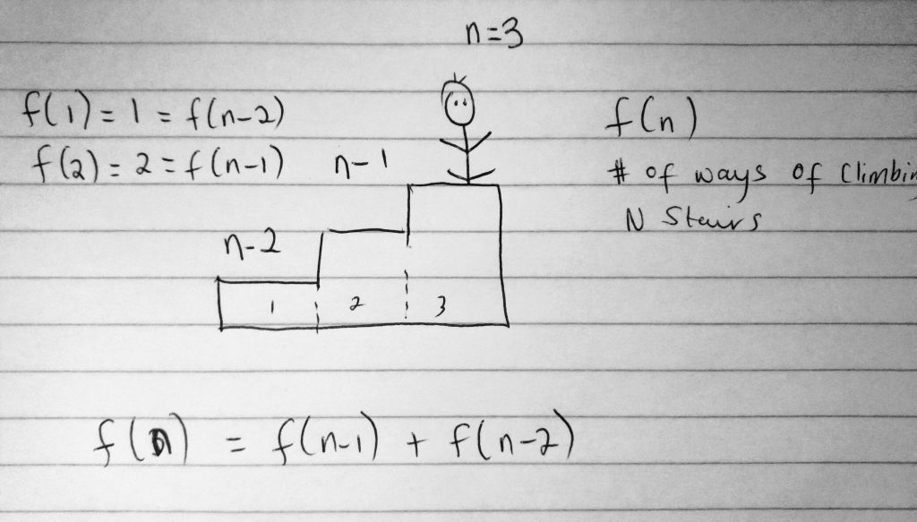
In the code above I have 2 ways of solving this problem. The first way is the recursive approach. The other 2 methods are using the dynamic programming approach. I have provided the recursive approach just so you can compare for yourself. Besides if you have the recursive solution, it sometimes makes it easier to solve using the dynamic programming. I won’t be going over the recursive code in this post, but you can look at the code. Lets look at the number of ways one can climb 3 stairs if they can only take one or 2 steps at a time.

In the above diagram we some 3 staircases. A good way of approaching such questions is to make a general assumption. In here we say, let f(n) be the number of ways to climb N stairs. If this is true, then to climb 3 stairs it would be f(3). If you had 3 stairs and it takes f(3) to climb 3 stairs, then it takes f(n-1) ways to reach the 2nd staircase and f(n-2) ways to reach the first staircase. It is only fair to say that f(3) = f(n – 1) + f(n – 2). This means that the number of ways to reach the 3 stairs is the total number of ways to reach the 1st step plus the total number of ways to reach the second step.

We are making these assumptions so we can define our base case(s). Which is very important if you are going to solve problems using this approach. Now let’s just say that you are on the (n – 2)th staircase (the first one). How many ways can you get to that step given the rules? Well, there is only 1 way if we count. f(1) = 1. What about the second staircase? Well, you can either go one step at a time ( 1 step and 1 step) or you can take 2 step at once. This makes it a total of 2 ways to climb 2 stairs given our rules ( f(2) = 2 ). In our code, we define our base cases. With that defined we are able to use the first 2 cases to build values that are next cases will use.

The next method adds an extra step to how we can climb stairs. We are not limited to either 1 or 2, we can take 3 steps at a time this time. In this case, it means that if we added a 3rd base case f(3) we get 4 ways of climbing 3 staircases given our rules. The first way is 1 step at a time. The second way is to climb one step then 2 steps. Third way is climb 2 steps then one 1. The final and fourth way is to just climb 3 step at a time for 1 time. Making a total of 4. We define this base case. We also change our general formula to be f(n) = f(n – 1) + f(n – 2) +  f(n – 3). Let’s solve more questions.

Cutting Rods

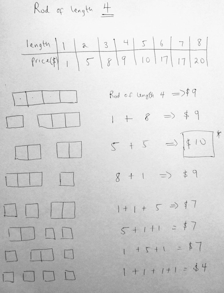
In this section, we are going to see how we can use dynamic programming to solve maximization problems. The question goes like this; given a rod of a certain length, along with prices for those lengths selling on the market, find out how to cut the rod so you can maximize the profit. The best way to start this problem is to use real-world examples. Let’s say we start by defining possible rod lengths with their prices in a table. So let’s see this looks like if we wanted to find the max profit of a rod of size 4.

In the diagram above we have a rod of length 4. We also see the market prices for rods given their length. A rod of length 4 is $9. How can we cut this rod to give us the maximum amount of profit? As you can see from the diagram, cutting the rod into 2 parts gives us a max of 10 dollars. Reason being a rod of length 2 is 5 dollars. You can see right away from this problem that finding the profit involves splitting the rods up and finding that profit, which leads us to think of a recursive solution(splitting up into smaller subproblems). Let’s come up with a general formula for this problem if possible. Take a look at this diagram:

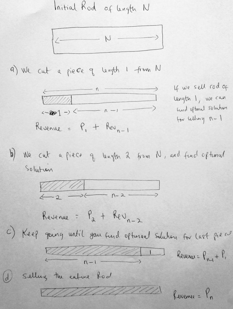
It starts off by cutting one piece of the road and sell it at any given price. Based on that price you are able to determine how to sell the remaining. In the diagram, given a rod of length N, we cut one unit out for a price P1. Then we find the optimal profit of the remaining based on what we sold one unit as. In figure a, the total revenue we can get from the rod is the price of selling one unit P1, plus the revenue we can make from selling the rest Rev(n – 1). We could have decided to cut the rod into 2 units and based on the price determined, calculate the revenue from the rod (see b in the diagram). We can keep doing this for different N units of rod until we get to C) when the remaining unit price is already known. Finally, we can sell the entire road as one piece of revenue Pn. As we experiment with this options, whichever one gives us the best profit is the one we choose.

Here is what our recursive solution will look like. Whichever one returns the max profit is the one we choose. Our base case is when we have a rod of zero length. That’s simple enough, the revenue there is zero dollars. So given the length of the rod with possible prices, we can find max revenue. This is how we are going to write our recursive code. From there we will come up with a dynamic programming solution. Let’s take a look at the recursive approach first.

See the Pen Cutting Rods – Javascript by kofi (@scriptonian) on CodePen.

In the code, we define a TotalRevenue function along with the length of the rod and the prices we want to find maximum profit or revenue for. The prices are defined within an array. We define a rod a length 4 like we did in a previous diagram along with prices representing each unit. So for 1 unit, it’s $1, for 2 units it’s $5, etc. In our function body, we define our base case. When the rod length is 0, the profit or revenue there is 0. We also define two other variables. The current revenue, which will represent the current revenue returned from the for-loop. We return whatever that max value as our final revenue. Running this function for a rod of length 4 we get $10. Just like we saw in the diagram. So our function is working! The only problem here is that since this is a recursive solution we find ourselves having exponential runtimes for large inputs. Let’s talk about what is going on in the dynamic programming approach. This function is called TotalRevenueDP. Again we start by defining our base case. From there we enter into a nested for-loop that returns the revenue of a rod with length 1, which we store so it can be used in the next iteration. Notice how our outer loop is set up. We start from 1 to rLen. We do this so we can set r[i] which will make it easier for us to solve the problem in the next iteration. The inner loop is the meat of the operation and does the actual calculation which we get by getting the price in the array and adding it the revenue of the previous operation. Please take a look at the code. Let’s look at the next question.

House Robber

You have N houses with a certain amount of money stashed in each house. You can not steal any adjacent houses (this only means that you cannot steal from houses that are next to each other). Given a list of non-negative integers representing the amount of money in each house, determine the maximum amount of money you can steal.

Let’s dive deeper into whats going on in this problem. Let’s just say that we can represent the amount of money for each house in an array [10, 20, 30, 40, 50]. Where the numbers in the array are the dollar amount for each house (first to the fifth house). We also know that you can not steal from adjacent houses (let’s just say when you do, the cops get alerts by some kind of security system). This means that you can only steal from houses in combinations such as:

[10, 30, 50]
[20, 40]
[10, 30]
[10, 40]
…

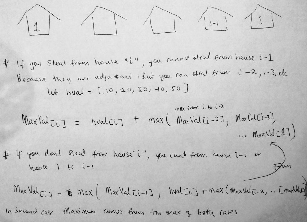
There are quite a lot ways you could steal without triggering any alerts (you could also skip more than 1 number). We can already see some patterns here. That there can be an order to the way houses can be robbed. Let’s take a look at a diagram

So we want to come up with a generalization of what it involves to steal a house from 1 to i. Two things can happen when we decide to do this. Either we steal house “i” as part of the process, or we don’t steal “i” at all. The reason is if we have stolen “i – 1” then we cant steal “i” because they are adjacent to each other. In the diagram above we try to come up with a formula. The MaxVal is the max value stolen so far on reaching house “i”. So in the first case if we steal house “i” then the max value is the value of the house at “i”, PLUS the max value from 1 to say “i – 2”, “i – 3”, etc. That should be fairly easy to understand. If we do not steal house “i”, then the max value we are looking for is house value at “i – 1” or the from 1 to “i – 1”, in comparison to what the value would be if we stole house “i” (which we already spoke about). So the second formula looks a bit confusing, but the second value being passed to the Math.max function is the same as the first formula. Note: The maximum of both options (steal from house “i” or not), is the solution for both cases.

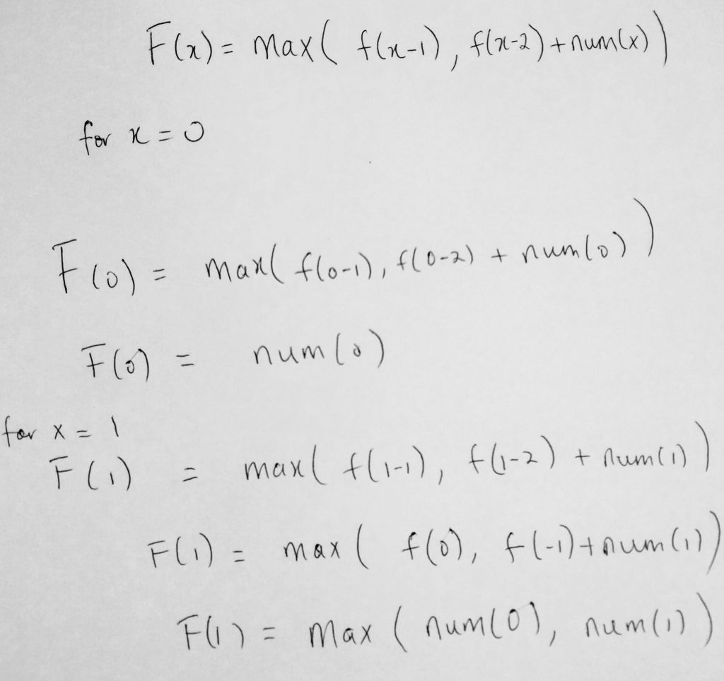
Let’s take a look at another way of viewing this formula using Math functions.

The formula above represents the solution of both cases (steal from house “i” or not). It is much easier to look at two formulas, but this one formula is condensed. What makes this version simple is that we can plug in values for x to see what the outcome is. For x = 0, we get the value in the num array (which is the price at index 0). You can look at this as a base case for when there is only one house. All we do is return the value at index zero. If there are 2 houses, we return the bigger of num[0] or num[1]. We use this in our code. Let’s take a look at both the recursive and dynamic solution for this problem.

See the Pen House Robber by kofi (@scriptonian) on CodePen.

Again I have provided multiple solutions. All solutions go through a process of finding out what the max value if house “i” is robbed or not. You can think of this also in terms of even and odd numbers. Since you cannot have an even numbered house that is robbed next to an odd number house that was also robbed. The recursive solution starts off by calling the rob function recursively for when house “i” is not robbed (count – 1). If there are 5 houses and we don’t start on the 5th house (which is “i”) then we are on a use-case where “i” is not robbed. We call the function until we get the base case (which returns nums[0]), and then we compare that to the max value that is returned if we called the function for house “i” being robbed. Also, it is important to take note of the base case.  If no houses are passed into the function, or the count of the houses is zero, we simply return 0 as the max value. If the count is 1, then we return the first value in the array as the max.

Next the dynamic programming solution. Notice how we build our table. The first index is the value of the first house, the second is the max of the first and the second. Then we run a for-loop from i = 2 to the last house and fill in our table with the necessary values. By the time we get to the end, we would have solved the problem (with the final answer being the last element in the table). This is so much simpler to understand than the recursive solution.

The final solution I provide is neither recursive nor dynamic programming. However, it makes it dead simple to understand. I also think that its probably the most intuitive way of approaching this problem. Do take a look at it. I will not be covering that in this post as I want to focus on dynamic programming.

Buy/Sell Stock to Maximize Profit

Our next problem falls under optimization problems that maximize the area of a field. In this case, buying stock. The problem goes like this: The cost of a stock on each day is given in an array (where the ith element is the price at that day). You are only allowed one transaction a day (buy one and sell one). Find the max profit you can make.

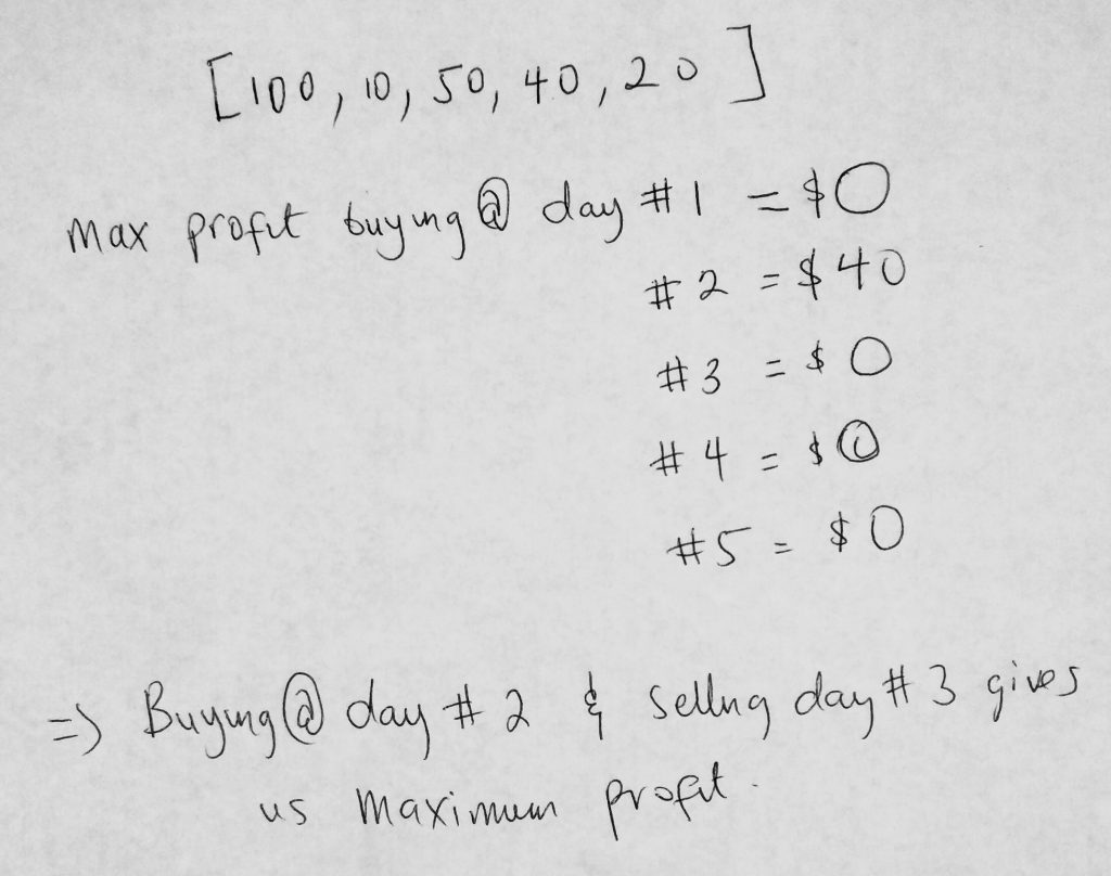
To start off the problem lets take our own sample dataset and see how profits can be made. Take a look at this diagram.

We are given a sample data of stock prices at day ” i ” ( [100, 10, 50, 40, 20] ). If we bought the stock on day 1 @ $100 dollars and sold it the second day, do we make a profit? No, we would have lost $90. In this case, if we sold at day 2 (which is i) we make a loss. We don’t want that, we want to maximize our profits. We can move iteratively through the given sample set and notice that if we buy at day 2 @$10 and sell at day 3 @$50, we make a profit of $40. Nothing else gives us profit that is as great. Let’s look at a diagram that will help us come up with a recursive solution.

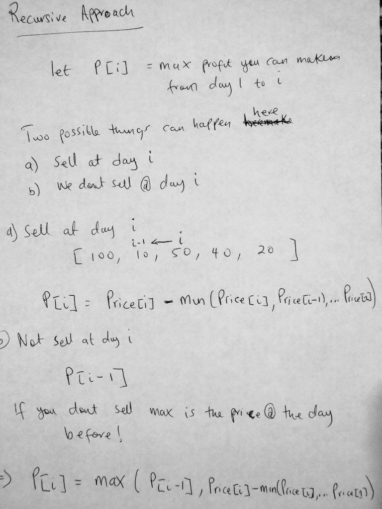
In the diagram we let P[i] represent the maximum profit we can make from day 1 to day i. Two things are possible we at day i. We either sell the stock or we don’t. If we sell the stock at say day 3, then we find how much profit we have made by traveling backward ([i – 1], [i – 2], etc) until we get to a day where the price was small enough to give us a profit. So we generalize the formula for a day we buy like this

P[i] = Price[i] – min( Price[i], Price[i – 1], Price[i – 2], …, Price[1] ) 

This is a simple formula. The maximum profit is the price on the given day you want to sell, minus the minimum of all the prices from that day to the first 1 (whichever is the smallest). Makes sense? If you don’t sell on day “i”, then the max profit you could ever make is from day 1 to i – 1 (P[i – 1] ). If we combine both of them together we can get the maximum profit

P[i] = max( P[i – 1], Price[i] – min( Price[i], Price[i – 1], Price[i – 2], …, Price[1] )  )

Get it? We have combined our two formulas and whichever is the maximum. Ok, let’s begin to take a look at how we are going to implement this in javascript.

See the Pen Buy / Sell Stock – Javascript by kofi (@scriptonian) on CodePen.

Ok, let’s have a look at the code above. There are 3 methods implemented ( one recursive and 2 dynamic programming ). I have 2 solutions for DP as one of them is more optimized. It turns out even using dynamic programming you can still end up with a runtime complexity of O(n^2). So the final method still uses DP but with a few tricks to give it a better runtime. So we have a general idea of what the question is and how to go about solving it (mathematical approach). In the code, you see that I have defined a few stock datasets (sample a, b & c). We also have a variable for days. Don’t forget that the dataset represents the amount of stock bought on day “i”. So the first value in the array represents the stock bought on day 1. The first method is the recursive approach. We define our base case. This is when we return zero if the number of days passed into the function is 0. If not we recursively call the function until an initial maximum value is found. Once we find a max value we loop through all the dataset from day 1 to the days passed into the function. Here we are able to find the new maximum value because we get to compare it to all other prices from subsequent days. Finally, we return the max value. The first dynamic programming approach is similar to the recursive approach but uses arrays (table) to store its initial revenue at day 0. Rv here is the same as the max value from the previous method. Remember at the end of the day when the function is done executing, what we want to do is return the maximum profit. Notice that when we start our outer loop we make an attempt to get the revenue located in the next slot of the table Rv[i], where i is day one initially. We run an inner loop which helps us make a comparison to all previous revenue values in order to come up with a max value. In the optimized approached, which is the 3 method, we try to avoid always going through the entire iteration when we have done it already. What we do is we store that value in a variable called minimum value, which we access later. Because of this, we have only one loop in our optimized method versus 2 in the inefficient method. Please take a look at the two methods for further clarification. Let’s move on!

Maximum Length Chain of Pairs

Our next example goes a little something like this: You are given n pairs of numbers. In every pair, the first number is always smaller than the second number. A pair (c, d) can follow another pair (a, b) if b < c. Chain of pairs can be formed in this fashion. Find the longest chain which can be formed from a given set of pairs.

Now let’s try to go a little bit into the details of what this question is asking. Lets just say we are given 3 pairs of number [ [3, 4], [4, 5], [5, 6] ]. Looking at the problem statement, a chain of pair (c, d) can follow pair (a, b) if b is less than c. Looking at the sample set, the second pair [4, 5] cannot follow [3, 4] because 4 is not greater than 4. So we skip that pair, which makes the longest change [3, 4] -> [5, 6]. In this case, 4 is less than 5 so they it can follow the chain.

If elements are in a chain for example (a, b) -> (c, d)

Then we can conclude a < b < c < d

Just like in our example above : 3 < 4 < 5 < 6

One way of going about this problem is sorting the pairs. First, we sort first number (a) for all the pairs, then we sort the second number (b) for all the pairs. We will create a utility class called Pair, which will be used for creating our pairs. Once done we will sort the “a” property first for the entire collection then the b property after that. Take this example, say after sorting we have this

sample set: [ [3, 4], [4, 5], [5, 6], [6, 7] ]

In the case, we started at pair 1 which is [3, 4] and ended on pair “i”, which is [6, 7]. Two things are possible. That

1. The longest chain ends on the ith pair
2. The longest chain does not end on the ith pair

Now in the case of #1, we are saying that if the longest chain ends on the ith pair, we can assume that the ith pair is one of the counts (i.e 1). The longest chain is a count of the number of pairs. In the sample set above let’s just say the first set is [3, 4] and i is [6, 7]. Let’s say “a” is the longest chain from 1 to a where a is [4, 5]. And “b” is [5, 6].

For #1 we can come up with a general formula like this

R[i] = Math.max(1 + R[a], 1 + R[b], 1 + R[c], …)

Remember that a, b and c must follow the rules of our inequality. a < b < c < d. So the above formula can be applied to find the longest chain if the chain ends in pair i.

In the second case, if the longest chain doesn’t end on pair “i”, then it means it ends on i – 1

R[i] = R[i – 1]

This means the longest chain is from 1 all the way to the (i – 1)th element.

When we put this together we get a general formula

R[i] = Math.max(R[i – 1], 1 + R[a], 1 + R[b], 1 + R[c], …)

This combines both cases and finds whichever is the max. Getting a bit confusing? Lets write some code.

See the Pen Maximum Length Chain Pair by kofi (@scriptonian) on CodePen.

Let’s take a look at what is going on here. First, let us state the obvious. We have a utility class called Pair, we use this to create our pair collection. Pairs are created with 2 properties which represent the elements in the pair, for eg [2, 3]. 2 is the first element and 3 is the second. We also have a custom sorting function which will help us sort our pair collection. We create some pairs using the pair constructor and pass it into our maximumLength function (which is where the main functionality live). The steps in the main function are not that complicated. First, we sort our collection using the firstElement column. We then do something interesting, which involves counting the pairs by adding the count number to an array. We do this so when we exit the function we can return that final number. We create 2 for loops, the first or outer loop goes through the sorted collection, whiles the inner loop is what adds the count to the table array. Since we are counting for the max and want to ensure that our previously defined inequality rules (a < b < d < d) hold we check to make sure that once the inner loops second element is less than the other loops first element [1, 2][2, 3][3, 4] (in this case making sure the second element of [1, 2] which is 2 is less than the first element of [2, 3]). If it is we add the incremented max to the table. Finally, we return that max value. Ok, let move into other territories with dynamic programming.

0 – 1 Knapsack Problem

The 0/1 knapsack problem is a famous one. The question can be presented in many different ways, but this is the version I like best. You are a thief with a knapsack that can carry X pounds of good. For lack of a better example, let’s just say the knapsack can carry a maximum of 20 pounds. You are in a store with a ton of stuff you can steal. The only limitation here is you can only steal what can fit in your knapsack. Use dynamic programming to write an algorithm that will maximize the number of items you can steal. Now its worth understanding why this is called 0 -1 knapsack problem. 0 – 1 means you can either pick an item or you don’t. This is a discrete knapsack problem. You either take all of an item or none of it. Now, why is this important? There are cases where the items you can steal are continuous. Like, say half a bread if it was food you were robbing. But you cannot take half a television. 0 -1 knacksack is used in the cases where you either take the whole of an item or you don’t. In the next post when we talk about greedy algorithms, we will look at fractional knapsack problems when you don’t have to take the whole of an item. You can take a fraction of it. More about that later.

Let’s look a little closer at this problem before we try to solve it. Imagine that there are 3 times you wanted to steal, given a knapsack that can hold only 20 pounds of items. A laptop which weighs 5 lbs and costs $4000, a digital keyboard that weight 10 pounds and costs $6000 and a home theater system that weighs 20 lbs and costs $9000. Which items would you choose? Well, we have not talked about greedy algorithms yet, but if you were very greedy then you would choose the item that is most expensive. This is what a greedy algorithm or person would do (we will learn about this in the next post). This may work but won’t give you the maximum value. This actually happens in the real world. We would just pick the most expensive on the list. The home system fits in our bag perfect and is the most expensive so why not. However if you were to pick the laptop and the keyboard, you would now be taking home $10,000 versus the $9000 for the home system. We are going to use dynamic programming to find the maximum value we can put in a knapsack given a set of items. To be more specific this problem falls under what we call 2-dimensional dynamic programming. Let’s take a look at a diagram.

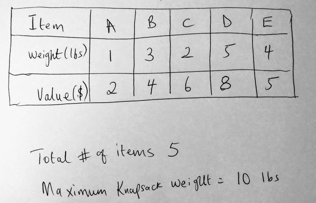
Let’s just say the problem at hand is what we see in the table. We have a total of 5 items (A, B, C, D, and E). The maximum amount of items we can put in our knapsack is 10 pounds. The table gives use data on the items we can steal (its weight and value). What we will do with this data is try to decide which items we put in our knapsack. First, let’s look at the recursive way (which is the slowest way). This way always involves trying every possible way to find out how to maximize profits. As we already know this way is not the most efficient. In every step of the way, we pick an item (say item A). Find out its weight and values and decide whether or not we are going to put it into our knapsack. So we make a yes or no decision. If its a yes, then its a 1 and a no is a 0 (zero) — hence the 0 – 1 knapsack problem. Let’s look at this 0 – 1 ( yes / no) in action by looking at another diagram.

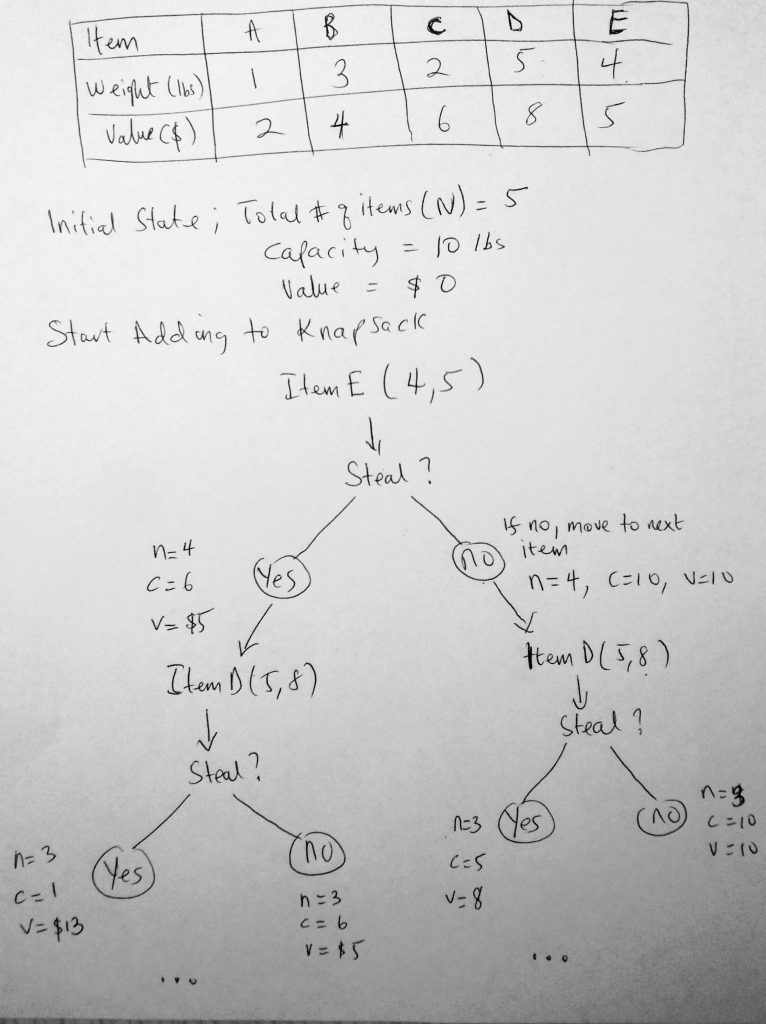
Let us start by looking at the recursive approach. We start at say the end of the list (at item E). We decide if we should steal this item. We go through the yes or no phase. If it’s a yes then we add it to the knapsack and update the remainder( capacity, value and remaining item count). We do the same for no. We keep doing this over and over again till we find the optimal solution. Lets us now write some code. We will first do it for the recursive approach and use dynamic programming to make it better.

See the Pen 0 – 1 Knapsack – Javascript by kofi (@scriptonian) on CodePen.

We start off with the recursive approach. We define our base-case; if the number of items or capacity is zero we simply set the final result variable to Zero. If you look at the diagram this makes sense. If you don’t choose any item to put in our knapsack, then what could you possibly expect to happen? However if the weight of the current item is greater than the capacity of our knapsack, then we cannot take that item. What do we is we move the next item on the list by calling the function again with (itemsNumber – 1) which is the item prior. If the item can however fit in our knapsack, then there are two things we can do. We put in our knapsack, or we don’t put it in our knapsack. Have you noticed this pattern or we either do this or that? We do it a lot in recursive/dynamic programming. Let’s move on. We find the maximum value of the two options (put in the knapsack or don’t). And that’s about it. We define an array of items and weights as well as the knapsack capacity and the total number of items. I would suggest you take a look at the code in GitHub, it has better commenting than you see in this post. We know that the recursive approach has a runtime of O(2 ^N) which is not good. So we move to the better dynamic programming approach. This method is strikingly similar to the recursive approach. However, we have introduced the array we normally do when working with DP problems. This will hold values for us so we don’t need to compute it again. The values we are holding in our 2D array stores the value of a number of items at a specific capacity, for example, array[0][1] will return 2. The 0 is the first position of the array and the 1 is the second item in that first array. Before we start storing any numbers notice that we initialized that dpArr. Next, when the function is run, we check to see if there is already a value for the current number of items being passed in and capacity. If this is not stored in our array then we move on to finding what the value is. However, note that we don’t call our function recursively many time. We call it at most 1 or 2 times when we want to find the max. That’s it! After that, the value will be stored in the array and can be retrieved easily. WHEW! Let’s move onto the next problem.

Longest Common Subsequence

The longest common subsequence or LCS has many useful applications. For example, it is very heavily used in molecular biology when doing DNA sequencing. Software engineering use “diff” to compare two different versions of the same file in order to see what has changed. This is all done with Longest Common Subsequence. Within our source code, we go through each line and display which ones have changed. It is also used in Screen redisplay (which is useful for slow terminal lines). Let’s take a look at examples through a diagram.

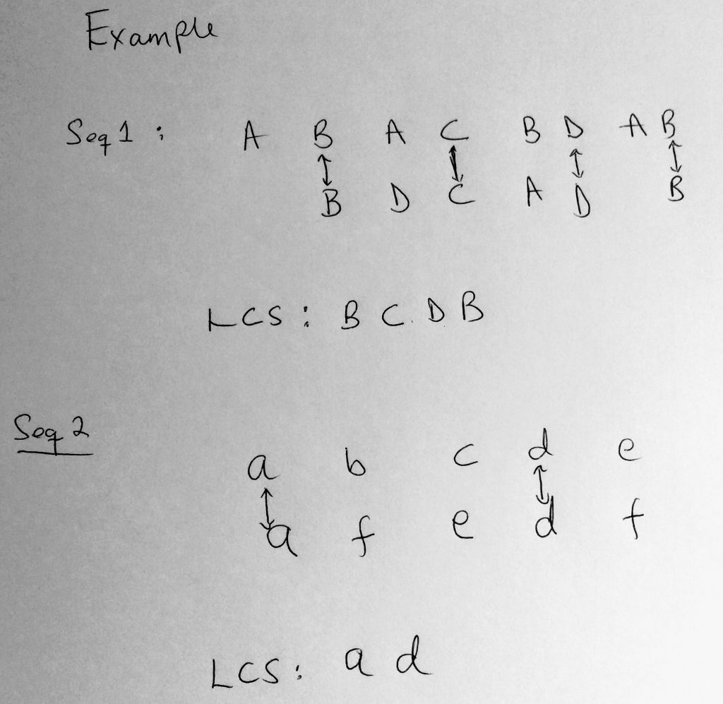
Above we have two examples that demonstrate what happens in LCS. In the first example, we have two strings. ABAC BDAB & BDC AD B. The spacing in the string doesn’t matter (they can be anything you want). The most important thing here is that we look for letter sequences. We noticed that in the first text we have a sequence of characters that follow the BCDB pattern. The second string also has this pattern. In this case, we return the length of the number of characters found, which is 4. In the second example, we do the same, A followed by D is found in both the first and second strings. We would return 2 in this case. Let dive a little deeper.

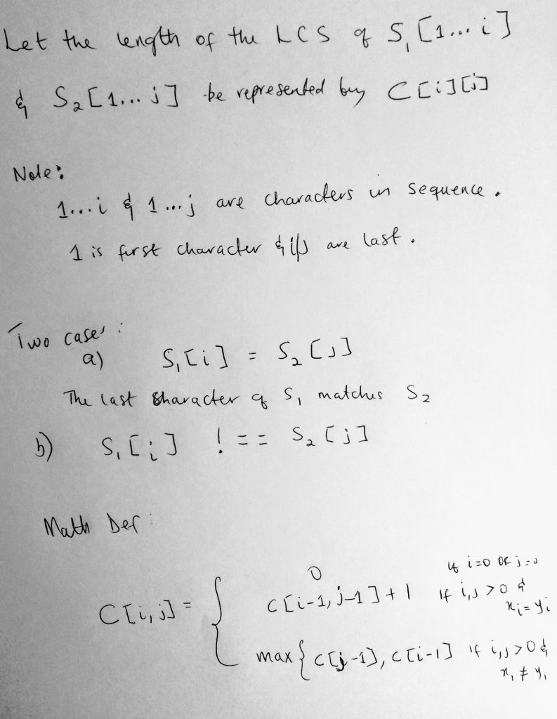
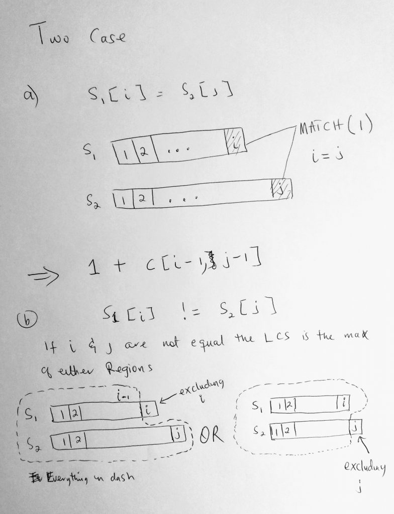
Here we try to come up with a general formula for getting what the LCS length. We define C[i][j] to represent the LCS of S1 (from 1 to i) and S2 (from 1 to j). So what does all this mean? Given a string (S1 or S2) we represent the number of characters within the string from 1 to the last character as 1 to “i” or. When we try to find this sequence given the string, two things are possible. The first is that you get two strings that have their last characters equal. For example, you get a string like “hello there I love to code” and “tell me when you are done”. Both strings end with the letter E. This is the first case. The second case is when the last letters are not equal. In that case here is what we do. First look at this diagram.

If the second case is true and the charters at the end don’t match, we find the LCS of the first string up until the last by one charter (so from 1 to (i – 1)) AND the LCS from 1 to j of the second string. Or we find the LCS of the first string from 1 to i AND from 1 to j – 1 of the second string. We find the max of the two (please look at the diagram for subregion). A math formula is also given on the image before. Now let’s write some code.

See the Pen Longest Common Subsequence – Javascript by kofi (@scriptonian) on CodePen.

Like we do in most cases I have provided 2 solutions. Let’s take a look at the first (the recursive approach). I hope by now you are familiar with this pattern. First, we define our base-case. We check to see if empty strings are passed to the function. If so we can immediately return zero. Next, we checking to see if the last characters of the strings passed in are equal. If they are then we have 1 match PLUS we recursive call the function again to finish up the count or store it in the final result. If the last characters are not matching then we do two recursive calls (one excluding the last charter of the first string and the other excluding the last character of the second string). I have already explained this, but here you find the code behind this logic. We find the maximum of these two and return the results. Also note that when we call LCS, we pass in the strings and their lengths. The dynamic solution part is just like we did the knapsack problem (2D dynamic programming). We initialize that array to a size of the small string (since the final number cannot be bigger than the length of that string). From here on when the function runs we first check to see if dpArr[m][n] already exists. If so we return that value (no need to call functions onto the stack). However, if the value is undefined or not in our table, we may make one or a max of 2 recursive calls (after when we store those values). Like the knapsack problem, this brings our runtime complexity to roughly O(N). OK, onto the next problem.

Longest Common Substring

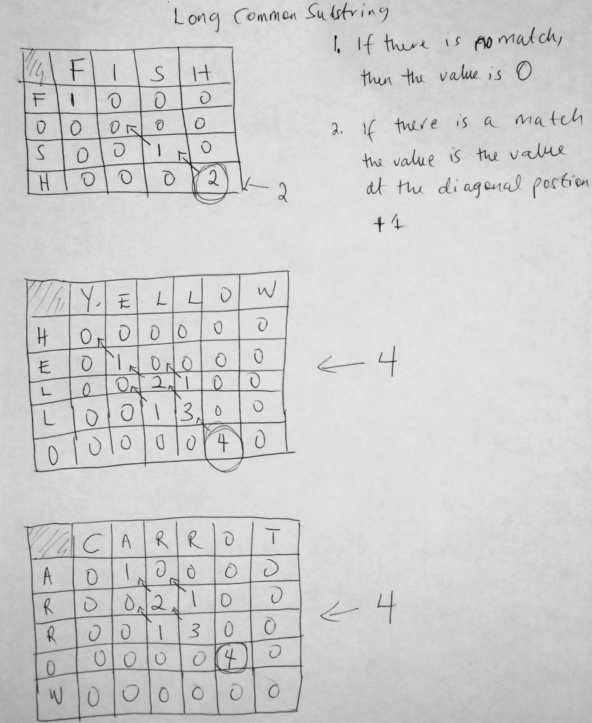
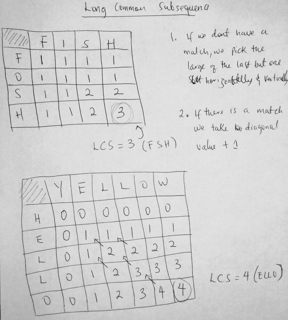
The next problem takes a somewhat similar to the previous. Given two strings S1 and S2, find the longest common substring between the two. Note that this is not to be confused with the subsequence approach we looked at before (which involves a sequence of characters). With longest common substring we need a continuous matching of a string(without any breaks). So for example given the words FISH and FOSH, the longest common subsequence is 3 (F, S & H), however, the longest common substring is 2 (S & H). Because S and H sit next to each other without any letters in between. We find the longest string that is a substring between the two strings. Let’s take a look at another example. What is the longest common substring between EAT and MEAT? Its 3 ( E, A, and T). What about “Hello” and “Yellow”? Its 4 ( ELLO). I think you get the picture.

In this example, I am going to show you how to solve this problem using tables. Matter of fact you could have used tables to solve the longest common subsequence problem. I will show you the table method for both. If you wish to go back to the previous problem and solve using this way (please feel free – and share that code with me!).

Every dynamic programming problem has a solution that involves a grid. We mentioned this earlier. The question is how do you use a table to solve the longest common subsequence and substring problem? Dynamic programming can be hard to understand (so practice is crucial). But from what we already know, it involves a grid with values. These values (in the table cells) are what we are trying to optimize to find out the solution. First, let me show you the table already filled out and we will go into the formula used to determine the final optimal answer. First the substring problem.

In the diagram above, there seems to be some weirdness going on. Somehow we are able to figure out what the longest common substring is by putting some values in our table. The formula is given. Here is how to apply it. You draw a table just like I have here. Starting from the string on the left, you go across horizontally for each letter. So here we started with the letter ‘A’. Then we go across horizontally. We try to match each letter in carrot. If the letters don’t match, we simply put a zero in that location. You can think of this table as a 2D array, where i and j are the rows and columns. If however there is a match, then we move to the value at the diagonal position and add 1 to it. Notice above that the diagonal position is represented by the arrow. Notice that when we get to the third row R, that when we find the first match, the diagonal value is 0. In that case, we add 1 to get 1. However, when we get to the second R match, the diagonal value is 2. So we add 1 to 2 and get 3. Simple isn’t it? Now let’s take a look at how to apply this to the longest common subsequence problem. It’s a little trickier.

Could you figure it out without the formula given on the paper? This one is tricky! Let me break it down to you. We create our table just like we did in a prior example. Again we go horizontally across the table starting from the H in ‘Hello’. When we check to see if H and Y matched, we notice that it didn’t. In the previous example, we automatically put zero. However, in this example, it is not always so. The value we put when there is no match is the value of the higher number before Y and H were reached. Since there wasn’t any it is zero. Its much better to understand starting from the second row E. When we found our first match, we did what we normally do. We add 1. However, notice that E and L that follow do not match however we have a one. Suppose that the value we are trying to figure out is X[i], where X[i] is the match between E and L. Horizontally the value because that slot is 1. Vertically the above is 0. Which is bigger? It’s 1. And we do this across. Think of it another way. We have a multidimensional array Cell[i][j] to represent this table. If we started from the first-row Cell[H][Y]. If there is a match we compute the value by Cell[H – 1][Y – 1] + 1. If there is no match, we find the max of Cell[H – 1][Y] and Cell[H][Y  – 1]. In the first row Cell[H – 1][Y] = 0 and Cell[H][Y  – 1] = 0. If you really want to get technical they are not defined so I just assigned 0. We could have used -1 (i think). I hope this is clear.

Let’s move back to the longest common substring problem and look at the code for it.

See the Pen Longest Common Substring – Javascript by kofi (@scriptonian) on CodePen.

Take a look at this beautiful code. From the formula we learned earlier on about how its applied to the substring problem, you can see everything clearly from the code. The first part of the code is a helper method I borrowed from Douglas Crockford. It’s a helper method that helps you create 2-dimensional arrays of any size as well as create it with initial values. So if I wanted to create a 4×4 array, or 3×5 or whatever size array, I can use this helper method to create it. It extends the javascript array class. This means we can call it on any array now. In the code, we define two strings. We also define their string size/length. We use this size to create a 2D array using the helper method. So if the string one was 4 characters and string two was 5 charters we create a 4×5 array. We pass the string and length values into our main function. Now here is where things look so simple. We have 2 for loops to represent our table. We run through each cell and apply the formula we have been talking about. If we find a match and it’s in the first row, we give it a value of 1, but if it’s not in that row then we take the diagonal value and add one. If there is no match we put zero in that place. As we do our iteration we save a value that is highest and return that value (which will be our LCS) at the end of the function! Sweet, there is nothing more to say. Let’s move on.

Maximum Sum Contiguous Subarray Problem

Here is the question: find the sum of contiguous subarray within an array (one-dimensional) of numbers which has the largest sum. The array should have at least one number.

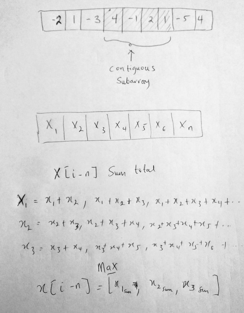
So what does all this mean? A contiguous subarray just means a subarray within an array that is continuous to a certain point. Perhaps an example will suffice. Given this array

[−2, 1, −3, 4, −1, 2, 1, −5, 4]

We can find a contiguous subarray within it [4, -1, 2, 1] that has the largest sum of 6. So all we are doing is scanning array for a set of numbers (which will also be an array), such that when you add then you get a maximum value. Let’s just say we start from the first element ( – 2 ). We keep adding numbers from -2 ( -2 + 1 = -1 ), or -2 + 1 + (-3) = =4. Note that this is starting from -2. After we are done we move to the next number and try to find the largest sum we can get by adding the numbers. Let’s take a look at a diagram

The diagram above shows you the subarray that is contiguous. As you can see the shaded region is what we call the subarray. So given this array, we want to find a subarray within it that its sum gives us the maximum value. Can you also see I have an array of X values from 1 (or i) to n. Let X[i – n] be the max value of the contiguous array. Then X[i – n] will be the max of calculating all the numbers sequentially as you see above.

So how would we code this? One possible way would be to go through all numbers in the array and add them. I think its best for you to look at the code. In our outer loop, we start from 0 to the last element on the array. Then we have 2 inner loops because we want to get to a position where we can start adding our numbers. We run a loop from i + 1 all the way to the end as our second loop. The final loop is what does the adding up. We move from i to j values and add them up. When we do we save that value as the current sum. In the end, we find the max of the previous maximum and the current sum. We keep doing this until we find a solution. Very nice! However, there is a problem. 3 for loops? That is not performant at all. That is O(N ^ 3) in time complexity. Another problem is that if all the numbers were negatives, we don’t get a correct answer. If you look in the GitHub repo, there is a solution for that. Can we do better than O(N ^ 3)? The answer is Yes. So let’s figure out how to make these improvements by looking at the code.

See the Pen Maximum Sum Contiguous Subarray Problem – Javascript by kofi (@scriptonian) on CodePen.

In the code, i have provided 3 examples. The first is the O(N ^ 3) solution. You can see how we are using 3 for loops to solve our problem. I will not go too much into details as i have already explained how this works, here is the code to back it up. What I will go into is how we improved the code. We can reduce our O(N ^ 3) solution to O(N)! which is a big improvement. What we do is we keep track of the current maximum as well as the total max. We start out by setting both of them to the first element in the array. We then loop to the end of our collection using the following rules: if the current sum during the iteration is less than zero, we set the current sum to zero, however, if the max sum is less than the current, then the max sum is the new current max. Take a look at the code. There is nothing earth-shattering that bare diving deeper into the code. At this level (advanced) things should be coming to you pretty intuitively.

This brings us to the end of our topic on dynamic programming. I really do hope that I have made it relatively easier for you to understand the topic through these examples (it’s not the easiest thing to just pick up). I suggest you answer more questions. The only way to get better at anything is to spend time on it. Solve many questions and before you know it, you are an expert on the topic. Lets now take a look at greedy algorithms.